
特征选择:11 种特征选择策略总结

来源:DeepHub IMBA 本文约4800字,建议阅读10+分钟
本文与你分享可应用于特征选择的各种技术的有用指南。
删除未使用的列 删除具有缺失值的列 不相关的特征 低方差特征 多重共线性 特征系数 p 值 方差膨胀因子 (VIF) 基于特征重要性的特征选择 使用 sci-kit learn 进行自动特征选择 主成分分析 (PCA)
import pandas as pddata = 'https://raw.githubusercontent.com/pycaret/pycaret/master/datasets/automobile.csv'df = pd.read_csv(data)df.sample(5)
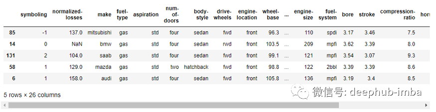
df.columns>> Index(['symboling', 'normalized-losses', 'make', 'fuel-type', 'aspiration', 'num-of-doors', 'body-style', 'drive-wheels', 'engine-location','wheel-base', 'length', 'width', 'height', 'curb-weight', 'engine-type', 'num-of-cylinders', 'engine-size', 'fuel-system', 'bore', 'stroke', 'compression-ratio', 'horsepower', 'peak-rpm', 'city-mpg', 'highway-mpg', 'price'], dtype='object')
现在让我们深入研究特征选择的 11 种策略。
删除未使用的列
删除具有缺失值的列
# total null values per columndf.isnull().sum()>>symboling 0normalized-losses 35make 0fuel-type 0aspiration 0num-of-doors 2body-style 0drive-wheels 0engine-location 0wheel-base 0length 0width 0height 0curb-weight 0engine-type 0num-of-cylinders 0engine-size 0fuel-system 0bore 0stroke 0compression-ratio 0horsepower 0peak-rpm 0city-mpg 0highway-mpg 0price 0dtype: int64
不相关的特征
# correlation between target and features(df.corr().loc['price'].plot(kind='barh', figsize=(4,10)))
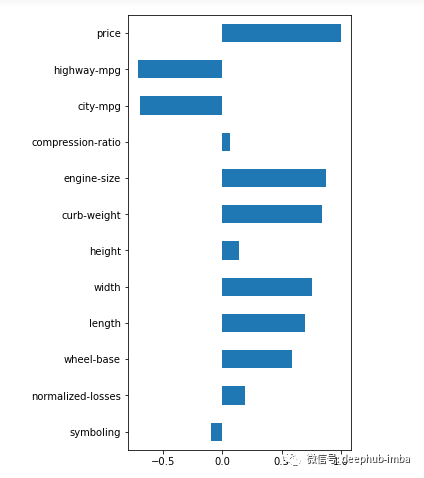
# drop uncorrelated numeric features (threshold <0.2)corr = abs(df.corr().loc['price'])corr = corr[corr<0.2]cols_to_drop = corr.index.to_list()df = df.drop(cols_to_drop, axis=1)
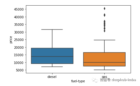
import seaborn as snssns.boxplot(y = 'price', x = 'fuel-type', data=df)
低方差特征
import numpy as np# variance of numeric features(df.select_dtypes(include=np.number).var().astype('str'))
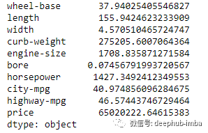
df['bore'].describe()
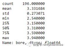
多重共线性
import matplotlib.pyplot as pltsns.set(rc={'figure.figsize':(16,10)})sns.heatmap(df.corr(),annot=True,linewidths=.5,center=0,cbar=False,cmap="PiYG")plt.show()
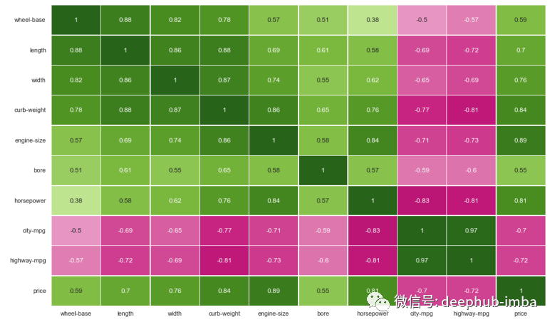
# drop correlated featuresdf = df.drop(['length', 'width', 'curb-weight', 'engine-size', 'city-mpg'], axis=1)
还可以使用称为方差膨胀因子 (VIF) 的方法来确定多重共线性并根据高 VIF 值删除特征。我稍后会展示这个例子。
df_cat = df[['fuel-type', 'body-style']]df_cat.sample(5)
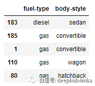
crosstab = pd.crosstab(df_cat['fuel-type'], df_cat['body-style'])crosstab
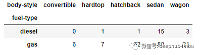
from scipy.stats import chi2_contingencychi2_contingency(crosstab)
# drop columns with missing valuesdf = df.dropna()from sklearn.model_selection import train_test_split# get dummies for categorical featuresdf = pd.get_dummies(df, drop_first=True)# X featuresX = df.drop('price', axis=1)# y targety = df['price']# split data into training and testing setX_train, X_test, y_train, y_test = train_test_split(X, y, test_size=0.3, random_state=42)from sklearn.linear_model import LinearRegression# scalingfrom sklearn.preprocessing import StandardScalerscaler = StandardScaler()X_train = scaler.fit_transform(X_train)X_test = scaler.fit_transform(X_test)# convert back to dataframeX_train = pd.DataFrame(X_train, columns = X.columns.to_list())X_test = pd.DataFrame(X_test, columns = X.columns.to_list())# instantiate modelmodel = LinearRegression()# fitmodel.fit(X_train, y_train)
特征系数
# feature coefficientscoeffs = model.coef_# visualizing coefficientsindex = X_train.columns.tolist()(pd.DataFrame(coeffs, index = index, columns = ['coeff']).sort_values(by = 'coeff').plot(kind='barh', figsize=(4,10)))
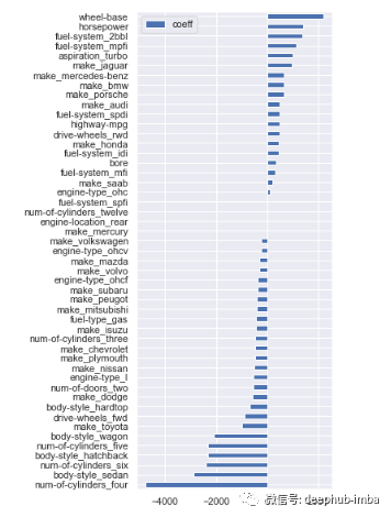
# filter variables near zero coefficient valuetemp = pd.DataFrame(coeffs, index = index, columns = ['coeff']).sort_values(by = 'coeff')temp = temp[(temp['coeff']>1) | (temp['coeff']< -1)]# drop those featurescols_coeff = temp.index.to_list()X_train = X_train[cols_coeff]X_test = X_test[cols_coeff]
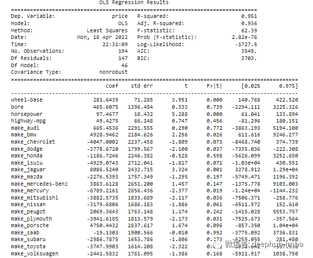
p 值
import statsmodels.api as smols = sm.OLS(y, X).fit()print(ols.summary())
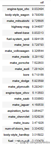
方差膨胀因子 (VIF)
VIF = 1 表示无相关性 VIF = 1-5 中等相关性 VIF >5 高相关
from statsmodels.stats.outliers_influence import variance_inflation_factor# calculate VIFvif = pd.Series([variance_inflation_factor(X.values, i) for i in range(X.shape[1])], index=X.columns)# display VIFs in a tableindex = X_train.columns.tolist()vif_df = pd.DataFrame(vif, index = index, columns = ['vif']).sort_values(by = 'vif', ascending=False)vif_df[vif_df['vif']<10]
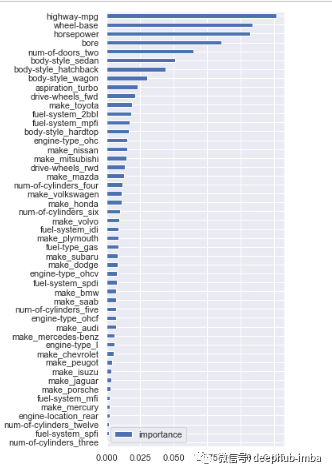
基于特征重要性选择
from sklearn.ensemble import RandomForestClassifier# instantiate modelmodel = RandomForestClassifier(n_estimators=200, random_state=0)# fit modelmodel.fit(X,y)
importances = model.feature_importances_cols = X.columns(pd.DataFrame(importances, cols, columns = ['importance']).sort_values(by='importance', ascending=True).plot(kind='barh', figsize=(4,10)))
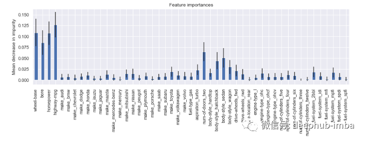
# calculate standard deviation of feature importancesstd = np.std([i.feature_importances_ for i in model.estimators_], axis=0)# visualizationfeat_with_importance = pd.Series(importances, X.columns)fig, ax = plt.subplots(figsize=(12,5))feat_with_importance.plot.bar(yerr=std, ax=ax)ax.set_title("Feature importances")ax.set_ylabel("Mean decrease in impurity")
使用 Scikit Learn 自动选择特征
# import modulesfrom sklearn.feature_selection import (SelectKBest, chi2, SelectPercentile, SelectFromModel, SequentialFeatureSelector, SequentialFeatureSelector)
基于卡方的技术
# select K best featuresX_best = SelectKBest(chi2, k=10).fit_transform(X,y)# number of best featuresX_best.shape[1]>> 10
# keep 75% top featuresX_top = SelectPercentile(chi2, percentile = 75).fit_transform(X,y)# number of best featuresX_top.shape[1]>> 36
# implement algorithmfrom sklearn.svm import LinearSVCmodel = LinearSVC(penalty= 'l1', C = 0.002, dual=False)model.fit(X,y)# select features using the meta transformerselector = SelectFromModel(estimator = model, prefit=True)X_new = selector.transform(X)X_new.shape[1]>> 2# names of selected featuresfeature_names = np.array(X.columns)feature_names[selector.get_support()]>> array(['wheel-base', 'horsepower'], dtype=object)
# instantiate modelmodel = RandomForestClassifier(n_estimators=100, random_state=0)# select featuresselector = SequentialFeatureSelector(estimator=model, n_features_to_select=10, direction='backward', cv=2)selector.fit_transform(X,y)# check names of features selectedfeature_names = np.array(X.columns)feature_names[selector.get_support()]>> array(['bore', 'make_mitsubishi', 'make_nissan', 'make_saab','aspiration_turbo', 'num-of-doors_two', 'body style_hatchback', 'engine-type_ohc', 'num-of-cylinders_twelve', 'fuel-system_spdi'], dtype=object)
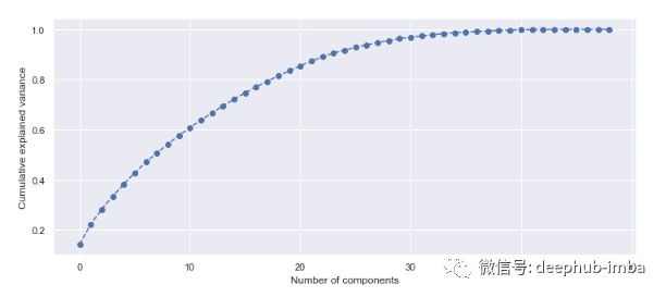
主成分分析 (PCA)
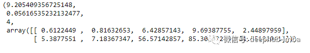
# import PCA modulefrom sklearn.decomposition import PCA# scaling dataX_scaled = scaler.fit_transform(X)# fit PCA to datapca = PCA()pca.fit(X_scaled)evr = pca.explained_variance_ratio_# visualizing the variance explained by each principal componentsplt.figure(figsize=(12, 5))plt.plot(range(0, len(evr)), evr.cumsum(), marker="o", linestyle="--")plt.xlabel("Number of components")plt.ylabel("Cumulative explained variance")
总结
评论