
基于Caret进行随机森林随机调参的4种方式
Caret是R中一个试图流程化机器学习方法的包,前面已有过介绍。
基于Caret进行随机森林随机调参
Caret只给randomForest函数提供了一个可调节参数mtry,即决策时的变量数目。随机调参就是函数会随机选取一些符合条件的参数值,逐个去尝试哪个可以获得更好的效果。
tuneLnegth设置随机选取的参数值的数目。metric设置模型评估标准,分类问题用Accuracy和Kappa值。也可以设置ROC (在第4章caret部分有讲解)。
if(file.exists('rda/rf_random.rda')){
  rf_random <- readRDS("rda/rf_random.rda")
} else {
  # Create model with default parameters
  trControl <- trainControl(method="repeatedcv", number=10, repeats=3, search="random")


  # 设置随机数种子,使得结果可重复
  seed <- 1
  set.seed(seed)

  rf_random <- train(x=expr_mat, y=metadata[[group]], method="rf",
                     tuneLength = 15, # 随机15个参数值或参数值组合
                     metric="Accuracy", #metric='Kappa'
                     trControl=trControl)
  saveRDS(rf_random, "rda/rf_random.rda")
}
print(rf_random)
## Random Forest
##
## 77 samples
## 7070 predictors
## 2 classes: 'DLBCL', 'FL'
##
## No pre-processing
## Resampling: Cross-Validated (10 fold, repeated 3 times)
## Summary of sample sizes: 70, 69, 69, 70, 69, 69, ...
## Resampling results across tuning parameters:
##
## mtry Accuracy Kappa
## 270 0.8988095 0.6586786
## 330 0.8821429 0.6129643
## 597 0.8946429 0.6529643
## 1301 0.9077381 0.7020960
## 1533 0.8988095 0.6729643
## 2177 0.9119048 0.7154293
## 2347 0.8904762 0.6462976
## 3379 0.8898810 0.6379783
## 4050 0.8940476 0.6475021
## 4065 0.8904762 0.6469326
## 4567 0.8946429 0.6564564
## 4775 0.8815476 0.6202005
## 5026 0.8946429 0.6709195
## 5307 0.8857143 0.6297244
## 6070 0.8815476 0.6163910
##
## Accuracy was used to select the optimal model using the largest value.
## The final value used for the model was mtry = 2177.最佳模型是mtry = 2177。
基于Caret进行随机森林指定参数调参
使用tuneGrid指定需要调整的参数和参数值,参数名字需要与函数预留的调参参数名字一致。
if(file.exists('rda/rf_grid.rda')){
  rf_grid <- readRDS("rda/rf_grid.rda")
} else {
  # Create model with default parameters
  trControl <- trainControl(method="repeatedcv", number=10, repeats=3, search="grid")

  # 根据经验或感觉设置一些待查询的参数和参数值
  tuneGrid <- expand.grid(mtry=c(3,10,20,50,100,300,700,1000,2000))
  # 设置随机数种子,使得结果可重复
  seed <- 1
  set.seed(seed)

  rf_grid <- train(x=expr_mat, y=metadata[[group]], method="rf",
                     tuneGrid = tuneGrid, # 随机15个参数值或参数值组合
                     metric="Accuracy", #metric='Kappa'
                     trControl=trControl)
  saveRDS(rf_grid, "rda/rf_grid.rda")
}
print(rf_grid)
## Random Forest
##
## 77 samples
## 7070 predictors
## 2 classes: 'DLBCL', 'FL'
##
## No pre-processing
## Resampling: Cross-Validated (10 fold, repeated 3 times)
## Summary of sample sizes: 70, 69, 69, 70, 69, 69, ...
## Resampling results across tuning parameters:
##
## mtry Accuracy Kappa
## 3 0.7875000 0.1596078
## 10 0.8345238 0.3766667
## 20 0.8511905 0.4731884
## 50 0.8648810 0.5324041
## 100 0.8779762 0.5920119
## 300 0.8946429 0.6558215
## 700 0.9071429 0.7002659
## 1000 0.9029762 0.6824881
## 2000 0.9071429 0.6920119
##
## Accuracy was used to select the optimal model using the largest value.
## The final value used for the model was mtry = 700.最佳模型是mtry = 700。
调整Caret没有提供的参数
如果我们想调整的参数Caret没有提供,可以用下面的方式自己手动+Caret配合调参。
if(file.exists('rda/rf_manual.rda')){
results <- readRDS("rda/rf_manual.rda")
} else {
# Manual Search
trControl <- trainControl(method="repeatedcv", number=10, repeats=3, search="grid")
# 用默认值固定mtry
# tunegrid <- expand.grid(mtry=c(sqrt(ncol(expr_mat))))
tunegrid <- expand.grid(mtry=c(700))
# 定义模型列表,存储每一个模型评估结果
modellist <- list()
# 调整的参数是决策树的数量
for (ntree in c(500,700, 800, 1000)) {
set.seed(seed)
fit <- train(x=expr_mat, y=metadata[[group]], method="rf",
metric="Accuracy", tuneGrid=tunegrid,
trControl=trControl, ntree=ntree)
key <- toString(ntree)
modellist[[key]] <- fit
}
# compare results
results <- resamples(modellist)
saveRDS(results, "rda/rf_manual.rda")
}
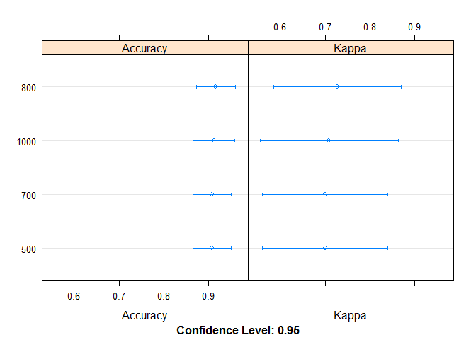
summary(results)##
## Call:
## summary.resamples(object = results)
##
## Models: 500, 700, 800, 1000
## Number of resamples: 30
##
## Accuracy
## Min. 1st Qu. Median Mean 3rd Qu. Max. NA's
## 500 0.5714286 0.875 0.9375 0.9071429 1 1 0
## 700 0.5714286 0.875 0.9375 0.9071429 1 1 0
## 800 0.5714286 0.875 1.0000 0.9154762 1 1 0
## 1000 0.5714286 0.875 1.0000 0.9113095 1 1 0
##
## Kappa
## Min. 1st Qu. Median Mean 3rd Qu. Max. NA's
## 500 -0.2352941 0.6 0.8571429 0.7002659 1 1 0
## 700 -0.2352941 0.6 0.8571429 0.7002659 1 1 0
## 800 -0.2352941 0.6 1.0000000 0.7269326 1 1 0
## 1000 -0.2352941 0.6 1.0000000 0.7091548 1 1 0绘制下图形
dotplot(results)800棵树时效果最好
扩展Caret
如果我们想调整的参数Caret没有提供,另一个方式是重新定义一个方法。尤其是参数比较多时,自己写循环会比较乱。
rf方法在Caret中的定义可通过此链接查看https://github.com/topepo/caret/blob/master/models/files/rf.R。需要做的修改就是在parameters上增加一个参数 (ntree),fit时调用下这个参数 (param$ntree)。
定义新方法
#  https://machinelearningmastery.com/tune-machine-learning-algorithms-in-r/
customRF <- list(type = "Classification", library = "randomForest", loop = NULL,
                 parameters = data.frame(parameter = c("mtry", "ntree"),
                                         class = rep("numeric", 2),
                                         label = c("mtry", "ntree")),

                  grid = function(x, y, len = NULL, search = "grid") {
                    if(search == "grid") {
                      out <- expand.grid(mtry = caret::var_seq(p = ncol(x),
                                                              classification = is.factor(y),
                                                              len = len),
                                         ntree = c(500,700,900,1000,1500))
                    } else {
                      out <- data.frame(mtry = unique(sample(1:ncol(x), size = len, replace = TRUE)),
                                        ntree = unique(sample(c(500,700,900,1000,1500),
                                                              size = len, replace = TRUE)))
                    }
                  },
                 fit = function(x, y, wts, param, lev, last, weights, classProbs, ...) {
                    randomForest(x, y, mtry = param$mtry, ntree=param$ntree, ...)
                  },
                predict = function(modelFit, newdata, preProc = NULL, submodels = NULL)
                  predict(modelFit, newdata),
                prob = function(modelFit, newdata, preProc = NULL, submodels = NULL)
                  predict(modelFit, newdata, type = "prob"),
                sort = function(x) x[order(x[,1]),],
                levels = function(x) x$classes
                )
调用新方法
# train model
if(file.exists('rda/rf_custom.rda')){
  rf_custom <- readRDS("rda/rf_custom.rda")
} else {
  trControl <- trainControl(method="repeatedcv", number=10, repeats=3)
  tunegrid <- expand.grid(mtry=c(3,10,20,50,100,300,700,1000,2000),
                          ntree=c(500,700, 800, 1000, 1500, 2000))
  set.seed(1)
  rf_custom <- train(x=expr_mat, y=metadata[[group]], method=customRF,
                   metric="Accuracy", tuneGrid=tunegrid,
                   trControl=trControl)
  saveRDS(rf_custom, "rda/rf_custom.rda")
}
print(rf_custom)
## 77 samples
## 7070 predictors
## 2 classes: 'DLBCL', 'FL'
##
## No pre-processing
## Resampling: Cross-Validated (10 fold, repeated 3 times)
## Summary of sample sizes: 70, 69, 69, 70, 69, 69, ...
## Resampling results across tuning parameters:
##
## mtry ntree Accuracy Kappa
## 3 500 0.7964286 0.1925490
## 3 700 0.7964286 0.1925490
## 3 800 0.7964286 0.1925490
## 3 1000 0.7922619 0.1792157
## 3 1500 0.7964286 0.1992157
## 3 2000 0.7922619 0.1792157
## 10 500 0.8083333 0.3000000
## 10 700 0.8220238 0.3233333
## 10 800 0.8214286 0.3225490
## 10 1000 0.8351190 0.3796078
## 10 1500 0.8303571 0.3566667
## 10 2000 0.8220238 0.3366667
## 20 500 0.8660714 0.5162745
## 20 700 0.8523810 0.4696078
## 20 800 0.8571429 0.4927962
## 20 1000 0.8351190 0.4061296
## 20 1500 0.8565476 0.4924041
## 20 2000 0.8517857 0.4727962
## 50 500 0.8744048 0.5531884
## 50 700 0.8648810 0.5428803
## 50 800 0.8702381 0.5465217
## 50 1000 0.8702381 0.5398551
## 50 1500 0.8702381 0.5398551
## 50 2000 0.8702381 0.5398551
## 100 500 0.8779762 0.5958215
## 100 700 0.8821429 0.6053453
## 100 800 0.8821429 0.5986786
## 100 1000 0.8952381 0.6398551
## 100 1500 0.8779762 0.5920119
## 100 2000 0.8869048 0.6131884
## 300 500 0.9029762 0.6720119
## 300 700 0.9029762 0.6758215
## 300 800 0.9071429 0.6920119
## 300 1000 0.8946429 0.6491548
## 300 1500 0.8988095 0.6624881
## 300 2000 0.8988095 0.6691548
## 700 500 0.9107143 0.7046450
## 700 700 0.9113095 0.7091548
## 700 800 0.9029762 0.6862976
## 700 1000 0.9071429 0.6920119
## 700 1500 0.9029762 0.6824881
## 700 2000 0.9071429 0.6958215
## 1000 500 0.9113095 0.7091548
## 1000 700 0.9029762 0.6824881
## 1000 800 0.9071429 0.6891548
## 1000 1000 0.9077381 0.7020960
## 1000 1500 0.9029762 0.6824881
## 1000 2000 0.9071429 0.6958215
## 2000 500 0.9029762 0.6824881
## 2000 700 0.9029762 0.6824881
## 2000 800 0.9119048 0.7116198
## 2000 1000 0.9029762 0.6824881
## 2000 1500 0.9029762 0.6824881
## 2000 2000 0.8988095 0.6691548
##
## Accuracy was used to select the optimal model using the largest value.
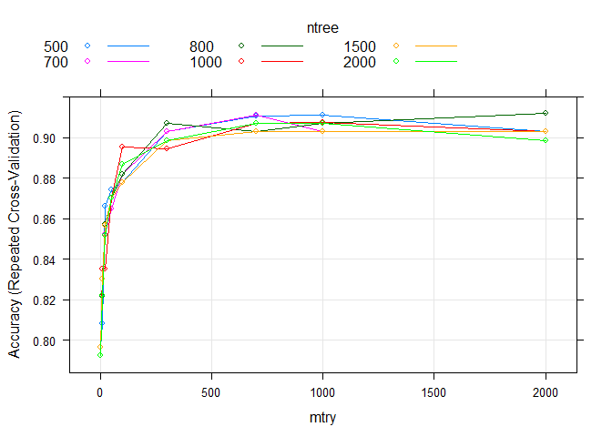
## The final values used for the model were mtry = 2000 and ntree = 800.绘制一张分布图
plot(rf_custom)同时评估mtry和ntree
References
官方文档 https://topepo.github.io/caret/model-training-and-tuning.html
部分中文解释 https://blog.csdn.net/weixin_42712867/article/details/105337052
特征选择 https://blog.csdn.net/jiabiao1602/article/details/44975741
调参的好例子 https://machinelearningmastery.com/tune-machine-learning-algorithms-in-r/
机器学习系列教程
从随机森林开始,一步步理解决策树、随机森林、ROC/AUC、数据集、交叉验证的概念和实践。
文字能说清的用文字、图片能展示的用、描述不清的用公式、公式还不清楚的写个简单代码,一步步理清各个环节和概念。
再到成熟代码应用、模型调参、模型比较、模型评估,学习整个机器学习需要用到的知识和技能。