用 Python 神经网络预测汽车保险支出-轻识

为新数据集开发神经网络预测模型可能具有挑战性。

一种方法是首先检查数据集并为可能使用的模型开发思路，然后探索数据集上简单模型的学习动态，然后最后使用健壮的测试工具为数据集开发和调整模型。此过程可用于为分类和回归预测建模问题开发有效的神经网络模型。

在本教程中，您将发现如何为瑞典汽车保险回归数据集开发多层Perceptron神经网络模型。完成本教程后，您将知道：

如何加载和汇总瑞典汽车保险数据集，以及如何使用结果建议要使用的数据准备和模型配置。
如何探索简单的MLP模型的学习动态以及数据集上的数据转换。
如何开发出对模型性能的可靠估计，调整模型性能以及对新数据进行预测。

教程概述

本教程分为四个部分。他们是：

汽车保险回归数据集
首个MLP和学习动力
评估和调整MLP模型
最终模型和做出预测

汽车保险回归数据集

第一步是定义和探索数据集。我们将使用“汽车保险”标准回归数据集。该数据集描述了瑞典的汽车保险。只有一个输入变量，即索赔的数量，目标变量是以数千瑞典克朗为单位的索赔总额。目的是在给定索赔数量的情况下预测总付款额。

您可以在此处了解有关数据集的更多信息：

汽车保险数据集（auto-insurance.csv）
汽车保险数据集详细信息（auto-insurance.names）

您可以在下面看到数据集的前几行。

108,392.5
19,46.2
13,15.7
124,422.2
40,119.4

我们可以看到这些值是数字的，范围从几十到几百。这表明在使用神经网络进行建模时，某种类型的缩放比例适合于数据。

我们可以直接从URL将数据集作为pandas DataFrame加载；例如：

# load the dataset and summarize the shape
from pandas import read_csv
# define the location of the dataset
url = 'https://raw.githubusercontent.com/jbrownlee/Datasets/master/auto-insurance.csv'
# load the dataset
df = read_csv(url, header=None)
# summarize shape
print(df.shape)

运行示例将直接从URL加载数据集并报告数据集的形状。

在这种情况下，我们可以确认该数据集具有两个变量（一个输入和一个输出），并且该数据集具有63行数据。

对于神经网络来说，这不是很多数据行，这表明一个小型的网络（可能带有正则化）将是合适的。

这也表明使用k倍交叉验证是一个好主意，因为与火车/测试拆分相比，它可以提供更可靠的模型性能估算值，并且因为单个模型可以在数秒而不是数小时或数天的时间内完成拟合。最大的数据集。

(63, 2)

接下来，我们可以通过查看摘要统计信息和数据图来了解有关数据集的更多信息。

# show summary statistics and plots of the dataset
from pandas import read_csv
from matplotlib import pyplot
# define the location of the dataset
url = 'https://raw.githubusercontent.com/jbrownlee/Datasets/master/auto-insurance.csv'
# load the dataset
df = read_csv(url, header=None)
# show summary statistics
print(df.describe())
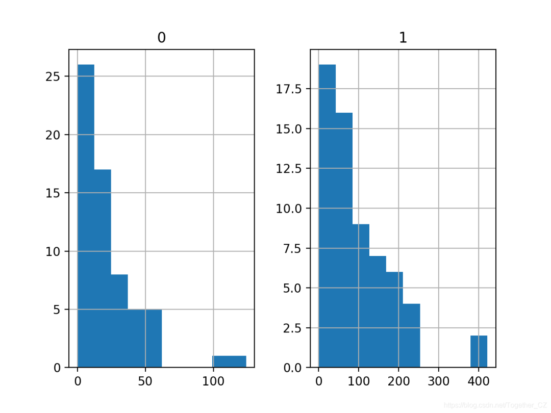
# plot histograms
df.hist()
pyplot.show()

运行示例之前，先加载数据，然后输出每个变量的摘要统计信息

我们可以看到每个变量的平均值在十个以内，范围从0到数百。这证实了缩放数据可能是一个好主意。

                0           1
count   63.000000   63.000000
mean    22.904762   98.187302
std     23.351946   87.327553
min      0.000000    0.000000
25%      7.500000   38.850000
50%     14.000000   73.400000
75%     29.000000  140.000000
max    124.000000  422.200000

然后为每个变量创建一个直方图。

我们可以看到每个变量都有相似的分布。它看起来像偏态的高斯分布或指数分布。

我们可以在每个变量上使用幂变换来降低概率分布的偏斜度，这可能会提高模型性能。

现在我们已经熟悉了数据集，让我们探讨如何开发神经网络模型。

首个MLP和学习动力

我们将使用TensorFlow为数据集开发一个多层感知器（MLP）模型。我们不知道学习超参数的哪种模型架构对这个数据集将是好的还是最好的，所以我们必须进行实验并发现什么是行之有效的。假设数据集很小，则小批量可能是个好主意，例如8或16行。入门时，使用Adam版本的随机梯度下降法是一个好主意，因为它会自动适应学习率，并且在大多数数据集上都能很好地工作。在认真评估模型之前，最好回顾一下学习动态并调整模型体系结构和学习配置，直到我们拥有稳定的学习动态，然后再充分利用模型。

我们可以通过简单的训练/测试数据拆分并查看学习曲线图来实现。这将帮助我们了解我们是学习过度还是学习不足；然后我们可以相应地调整配置。首先，我们可以将数据集分为输入和输出变量，然后分为67/33训练和测试集。

# split into input and output columns
X, y = df.values[:, :-1], df.values[:, -1]
# split into train and test datasets
X_train, X_test, y_train, y_test = train_test_split(X, y, test_size=0.33)

接下来，我们可以定义一个最小的MLP模型。在这种情况下，我们将使用一个包含10个节点的隐藏层和一个输出层（任意选择）。我们将在隐藏层中使用ReLU激活功能和“ he_normal”权重初始化，因为它们是一种很好的做法。

模型的输出是线性激活（不激活），我们将最小化均方误差（MSE）损失。

# determine the number of input features
n_features = X.shape[1]
# define model
model = Sequential()
model.add(Dense(10, activation='relu', kernel_initializer='he_normal', input_shape=(n_features,)))
model.add(Dense(1))
# compile the model
model.compile(optimizer='adam', loss='mse')

我们将模型拟合为100个训练时期（任意选择），批量为8个，因为它是一个很小的数据集。我们正在原始数据上拟合模型，我们认为这可能不是一个好主意，但这是一个重要的起点。

# fit the model
history = model.fit(X_train, y_train, epochs=100, batch_size=8, verbose=0, validation_data=(X_test,y_test))

在训练结束时，我们将评估模型在测试数据集上的性能，并将性能报告为平均绝对误差（MAE），我通常更喜欢MSE或RMSE。

# predict test set
yhat = model.predict(X_test)
# evaluate predictions
score = mean_absolute_error(y_test, yhat)
print('MAE: %.3f' % score)

最后，我们将在训练期间在训练和测试集上绘制MSE损失的学习曲线。

# plot learning curves
pyplot.title('Learning Curves')
pyplot.xlabel('Epoch')
pyplot.ylabel('Mean Squared Error')
pyplot.plot(history.history['loss'], label='train')
pyplot.plot(history.history['val_loss'], label='val')
pyplot.legend()
pyplot.show()

综上所述，下面列出了评估我们在汽车保险数据集上的第一个MLP的完整示例。

# fit a simple mlp model and review learning curves
from pandas import read_csv
from sklearn.model_selection import train_test_split
from sklearn.metrics import mean_absolute_error
from tensorflow.keras import Sequential
from tensorflow.keras.layers import Dense
from matplotlib import pyplot
# load the dataset
path = 'https://raw.githubusercontent.com/jbrownlee/Datasets/master/auto-insurance.csv'
df = read_csv(path, header=None)
# split into input and output columns
X, y = df.values[:, :-1], df.values[:, -1]
# split into train and test datasets
X_train, X_test, y_train, y_test = train_test_split(X, y, test_size=0.33)
# determine the number of input features
n_features = X.shape[1]
# define model
model = Sequential()
model.add(Dense(10, activation='relu', kernel_initializer='he_normal', input_shape=(n_features,)))
model.add(Dense(1))
# compile the model
model.compile(optimizer='adam', loss='mse')
# fit the model
history = model.fit(X_train, y_train, epochs=100, batch_size=8, verbose=0, validation_data=(X_test,y_test))
# predict test set
yhat = model.predict(X_test)
# evaluate predictions
score = mean_absolute_error(y_test, yhat)
print('MAE: %.3f' % score)
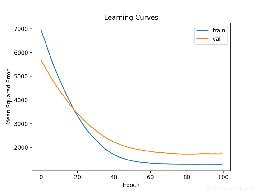
# plot learning curves
pyplot.title('Learning Curves')
pyplot.xlabel('Epoch')
pyplot.ylabel('Mean Squared Error')
pyplot.plot(history.history['loss'], label='train')
pyplot.plot(history.history['val_loss'], label='val')
pyplot.legend()
pyplot.show()

运行示例首先使模型适合训练数据集，然后报告测试数据集的MAE。

注意：由于算法或评估程序的随机性，或者数值精度的差异，您的结果可能会有所不同。考虑运行该示例几次并比较平均结果。

在这种情况下，我们可以看到该模型实现了大约33.2的MAE，这是性能的良好基准，我们可能可以对其进行改进。

MAE: 33.233

然后在火车和测试装置上创建MSE的线图。

我们可以看到该模型具有良好的拟合度，并且收敛良好。模型的配置是一个很好的起点。

到目前为止，学习动力很好，MAE是一个粗略的估计，不应该被依赖。

我们可能可以稍微增加模型的容量，并期待类似的学习动态。例如，我们可以添加具有八个节点（任意选择）的第二个隐藏层，并将训练时期数增加一倍至200。

# define model
model = Sequential()
model.add(Dense(10, activation='relu', kernel_initializer='he_normal', input_shape=(n_features,)))
model.add(Dense(8, activation='relu', kernel_initializer='he_normal'))
model.add(Dense(1))
# compile the model
model.compile(optimizer='adam', loss='mse')
# fit the model
history = model.fit(X_train, y_train, epochs=200, batch_size=8, verbose=0, validation_data=(X_test,y_test))

完整实例如下：

# fit a deeper mlp model and review learning curves
from pandas import read_csv
from sklearn.model_selection import train_test_split
from sklearn.metrics import mean_absolute_error
from tensorflow.keras import Sequential
from tensorflow.keras.layers import Dense
from matplotlib import pyplot
# load the dataset
path = 'https://raw.githubusercontent.com/jbrownlee/Datasets/master/auto-insurance.csv'
df = read_csv(path, header=None)
# split into input and output columns
X, y = df.values[:, :-1], df.values[:, -1]
# split into train and test datasets
X_train, X_test, y_train, y_test = train_test_split(X, y, test_size=0.33)
# determine the number of input features
n_features = X.shape[1]
# define model
model = Sequential()
model.add(Dense(10, activation='relu', kernel_initializer='he_normal', input_shape=(n_features,)))
model.add(Dense(8, activation='relu', kernel_initializer='he_normal'))
model.add(Dense(1))
# compile the model
model.compile(optimizer='adam', loss='mse')
# fit the model
history = model.fit(X_train, y_train, epochs=200, batch_size=8, verbose=0, validation_data=(X_test,y_test))
# predict test set
yhat = model.predict(X_test)
# evaluate predictions
score = mean_absolute_error(y_test, yhat)
print('MAE: %.3f' % score)
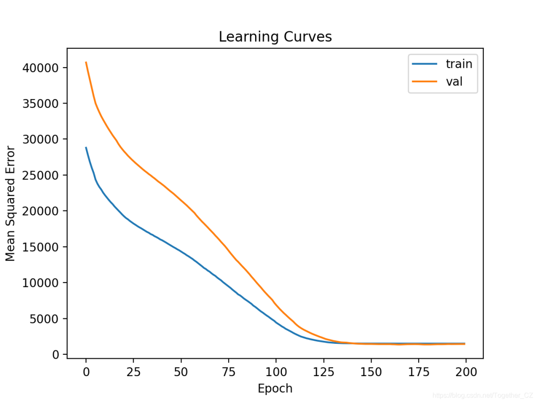
# plot learning curves
pyplot.title('Learning Curves')
pyplot.xlabel('Epoch')
pyplot.ylabel('Mean Squared Error')
pyplot.plot(history.history['loss'], label='train')
pyplot.plot(history.history['val_loss'], label='val')
pyplot.legend()
pyplot.show()

运行示例首先使模型适合训练数据集，然后报告测试数据集的MAE。

注意：由于算法或评估程序的随机性，或者数值精度的差异，您的结果可能会有所不同。考虑运行该示例几次并比较平均结果。

在这种情况下，我们可以看到MAE略有改善，约为27.9，尽管训练/测试拆分的高方差意味着该评估是不可靠的。

MAE: 27.939

然后绘制MSE训练和测试集的学习曲线。我们可以看到，正如预期的那样，该模型在合理的迭代次数内实现了良好的拟合和收敛。

最后，我们可以尝试转换数据，看看它如何影响学习动力。

在这种情况下，我们将使用幂变换来减少数据分布的偏差。这还将自动标准化变量，以使它们的平均值为零，标准偏差为1，这是使用神经网络进行建模时的一种好习惯。

首先，我们必须确保目标变量是二维数组。

# ensure that the target variable is a 2d array
y_train, y_test = y_train.reshape((len(y_train),1)), y_test.reshape((len(y_test),1))

接下来，我们可以将PowerTransformer应用于输入变量和目标变量。

这可以通过首先将转换适合训练数据，然后转换训练和测试集来实现。

此过程将分别应用于输入和输出变量，以避免数据泄漏。

# power transform input data
pt1 = PowerTransformer()
pt1.fit(X_train)
X_train = pt1.transform(X_train)
X_test = pt1.transform(X_test)
# power transform output data
pt2 = PowerTransformer()
pt2.fit(y_train)
y_train = pt2.transform(y_train)
y_test = pt2.transform(y_test)

然后将数据用于拟合模型。

后面可以根据模型做出的预测以及测试集中的预期目标值对变换进行求逆，我们可以像以前一样以正确的比例计算MAE。

# inverse transforms on target variable
y_test = pt2.inverse_transform(y_test)
yhat = pt2.inverse_transform(yhat)

结合在一起，下面列出了使用转换后的数据拟合和评估MLP以及创建模型的学习曲线的完整示例。

# fit a mlp model with data transforms and review learning curves
from pandas import read_csv
from sklearn.model_selection import train_test_split
from sklearn.metrics import mean_absolute_error
from sklearn.preprocessing import PowerTransformer
from tensorflow.keras import Sequential
from tensorflow.keras.layers import Dense
from matplotlib import pyplot
# load the dataset
path = 'https://raw.githubusercontent.com/jbrownlee/Datasets/master/auto-insurance.csv'
df = read_csv(path, header=None)
# split into input and output columns
X, y = df.values[:, :-1], df.values[:, -1]
# split into train and test datasets
X_train, X_test, y_train, y_test = train_test_split(X, y, test_size=0.33)
# ensure that the target variable is a 2d array
y_train, y_test = y_train.reshape((len(y_train),1)), y_test.reshape((len(y_test),1))
# power transform input data
pt1 = PowerTransformer()
pt1.fit(X_train)
X_train = pt1.transform(X_train)
X_test = pt1.transform(X_test)
# power transform output data
pt2 = PowerTransformer()
pt2.fit(y_train)
y_train = pt2.transform(y_train)
y_test = pt2.transform(y_test)
# determine the number of input features
n_features = X.shape[1]
# define model
model = Sequential()
model.add(Dense(10, activation='relu', kernel_initializer='he_normal', input_shape=(n_features,)))
model.add(Dense(8, activation='relu', kernel_initializer='he_normal'))
model.add(Dense(1))
# compile the model
model.compile(optimizer='adam', loss='mse')
# fit the model
history = model.fit(X_train, y_train, epochs=200, batch_size=8, verbose=0, validation_data=(X_test,y_test))
# predict test set
yhat = model.predict(X_test)
# inverse transforms on target variable
y_test = pt2.inverse_transform(y_test)
yhat = pt2.inverse_transform(yhat)
# evaluate predictions
score = mean_absolute_error(y_test, yhat)
print('MAE: %.3f' % score)
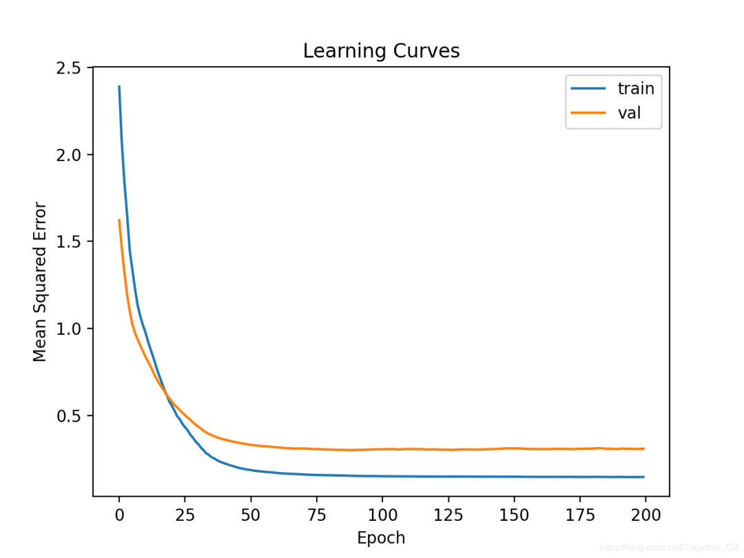
# plot learning curves
pyplot.title('Learning Curves')
pyplot.xlabel('Epoch')
pyplot.ylabel('Mean Squared Error')
pyplot.plot(history.history['loss'], label='train')
pyplot.plot(history.history['val_loss'], label='val')
pyplot.legend()
pyplot.show()

运行示例首先使模型适合训练数据集，然后报告测试数据集的MAE。

注意：由于算法或评估程序的随机性，或者数值精度的差异，您的结果可能会有所不同。考虑运行该示例几次并比较平均结果。

在这种情况下，该模型可以达到合理的MAE分数，尽管比以前报告的性能差。我们暂时将忽略模型性能。

MAE: 34.320

创建了学习曲线的线图，表明该模型达到了合理的拟合并且有足够的时间收敛。

现在，我们对带有或不带有数据转换的简单MLP模型的学习动态有了一些了解，现在我们可以看一下评估模型的性能以及调整模型的配置。

评估和调整MLP模型

k倍交叉验证过程可以提供更可靠的MLP性能估计，尽管它可能非常慢。这是因为必须拟合和评估k个模型。当数据集大小较小时（例如汽车保险数据集），这不是问题。我们可以使用KFold类创建拆分并手动枚举每个折叠，拟合模型，对其进行评估，然后在过程结束时报告评估分数的平均值。

# prepare cross validation
kfold = KFold(10)
# enumerate splits
scores = list()
for train_ix, test_ix in kfold.split(X, y):
 # fit and evaluate the model...
 ...
...
# summarize all scores
print('Mean MAE: %.3f (%.3f)' % (mean(scores), std(scores)))

我们可以使用此框架通过一系列不同的数据准备，模型架构和学习配置来开发MLP模型性能的可靠估计。

重要的是，在使用k-fold交叉验证来评估性能之前，我们首先对上一部分中的数据集模型的学习动态有了了解。如果我们开始直接调整模型，我们可能会获得良好的结果，但是如果没有，我们可能不知道为什么，例如模型超出或不足。

如果我们再次对模型进行较大的更改，则最好返回并确认模型正在适当收敛。

下面列出了评估上一节中的基本MLP模型的此框架的完整示例。

# k-fold cross-validation of base model for the auto insurance regression dataset
from numpy import mean
from numpy import std
from pandas import read_csv
from sklearn.model_selection import KFold
from sklearn.metrics import mean_absolute_error
from tensorflow.keras import Sequential
from tensorflow.keras.layers import Dense
from matplotlib import pyplot
# load the dataset
path = 'https://raw.githubusercontent.com/jbrownlee/Datasets/master/auto-insurance.csv'
df = read_csv(path, header=None)
# split into input and output columns
X, y = df.values[:, :-1], df.values[:, -1]
# prepare cross validation
kfold = KFold(10)
# enumerate splits
scores = list()
for train_ix, test_ix in kfold.split(X, y):
 # split data
 X_train, X_test, y_train, y_test = X[train_ix], X[test_ix], y[train_ix], y[test_ix]
 # determine the number of input features
 n_features = X.shape[1]
 # define model
 model = Sequential()
 model.add(Dense(10, activation='relu', kernel_initializer='he_normal', input_shape=(n_features,)))
 model.add(Dense(1))
 # compile the model
 model.compile(optimizer='adam', loss='mse')
 # fit the model
 model.fit(X_train, y_train, epochs=100, batch_size=8, verbose=0)
 # predict test set
 yhat = model.predict(X_test)
 # evaluate predictions
 score = mean_absolute_error(y_test, yhat)
 print('>%.3f' % score)
 scores.append(score)
# summarize all scores
print('Mean MAE: %.3f (%.3f)' % (mean(scores), std(scores)))

运行示例将在评估过程的每次迭代中报告模型性能，并在运行结束时报告MAE的平均值和标准偏差。

注意：由于算法或评估程序的随机性，或者数值精度的差异，您的结果可能会有所不同。考虑运行该示例几次并比较平均结果。

在这种情况下，我们可以看到MLP模型的MAE约为38.913。

我们将使用此结果作为基准，以查看是否可以实现更好的性能。

>27.314
>69.577
>20.891
>14.810
>13.412
>69.540
>25.612
>49.508
>35.769
>62.696
Mean MAE: 38.913 (21.056)

首先，让我们尝试在原始数据集上评估更深的模型，以查看其性能是否比基准模型更好。

# define model
model = Sequential()
model.add(Dense(10, activation='relu', kernel_initializer='he_normal', input_shape=(n_features,)))
model.add(Dense(8, activation='relu', kernel_initializer='he_normal'))
model.add(Dense(1))
# compile the model
model.compile(optimizer='adam', loss='mse')
# fit the model
model.fit(X_train, y_train, epochs=200, batch_size=8, verbose=0)

完整实例如下：

# k-fold cross-validation of deeper model for the auto insurance regression dataset
from numpy import mean
from numpy import std
from pandas import read_csv
from sklearn.model_selection import KFold
from sklearn.metrics import mean_absolute_error
from tensorflow.keras import Sequential
from tensorflow.keras.layers import Dense
from matplotlib import pyplot
# load the dataset
path = 'https://raw.githubusercontent.com/jbrownlee/Datasets/master/auto-insurance.csv'
df = read_csv(path, header=None)
# split into input and output columns
X, y = df.values[:, :-1], df.values[:, -1]
# prepare cross validation
kfold = KFold(10)
# enumerate splits
scores = list()
for train_ix, test_ix in kfold.split(X, y):
 # split data
 X_train, X_test, y_train, y_test = X[train_ix], X[test_ix], y[train_ix], y[test_ix]
 # determine the number of input features
 n_features = X.shape[1]
 # define model
 model = Sequential()
 model.add(Dense(10, activation='relu', kernel_initializer='he_normal', input_shape=(n_features,)))
 model.add(Dense(8, activation='relu', kernel_initializer='he_normal'))
 model.add(Dense(1))
 # compile the model
 model.compile(optimizer='adam', loss='mse')
 # fit the model
 model.fit(X_train, y_train, epochs=200, batch_size=8, verbose=0)
 # predict test set
 yhat = model.predict(X_test)
 # evaluate predictions
 score = mean_absolute_error(y_test, yhat)
 print('>%.3f' % score)
 scores.append(score)
# summarize all scores
print('Mean MAE: %.3f (%.3f)' % (mean(scores), std(scores)))

运行报告运行结束时MAE的平均值和标准偏差。

注意：由于算法或评估程序的随机性，或者数值精度的差异，您的结果可能会有所不同。考虑运行该示例几次并比较平均结果。

在这种情况下，我们可以看到MLP模型获得的MAE约为35.384，这略好于获得MAE约为38.913的基线模型。

Mean MAE: 35.384 (14.951)

接下来，让我们尝试使用与上一节相同的对输入和目标变量进行幂变换的模型。

下面列出了完整的示例。

# k-fold cross-validation of deeper model with data transforms
from numpy import mean
from numpy import std
from pandas import read_csv
from sklearn.model_selection import KFold
from sklearn.metrics import mean_absolute_error
from sklearn.preprocessing import PowerTransformer
from tensorflow.keras import Sequential
from tensorflow.keras.layers import Dense
from matplotlib import pyplot
# load the dataset
path = 'https://raw.githubusercontent.com/jbrownlee/Datasets/master/auto-insurance.csv'
df = read_csv(path, header=None)
# split into input and output columns
X, y = df.values[:, :-1], df.values[:, -1]
# prepare cross validation
kfold = KFold(10)
# enumerate splits
scores = list()
for train_ix, test_ix in kfold.split(X, y):
 # split data
 X_train, X_test, y_train, y_test = X[train_ix], X[test_ix], y[train_ix], y[test_ix]
 # ensure target is a 2d array
 y_train, y_test = y_train.reshape((len(y_train),1)), y_test.reshape((len(y_test),1))
 # prepare input data
 pt1 = PowerTransformer()
 pt1.fit(X_train)
 X_train = pt1.transform(X_train)
 X_test = pt1.transform(X_test)
 # prepare target
 pt2 = PowerTransformer()
 pt2.fit(y_train)
 y_train = pt2.transform(y_train)
 y_test = pt2.transform(y_test)
 # determine the number of input features
 n_features = X.shape[1]
 # define model
 model = Sequential()
 model.add(Dense(10, activation='relu', kernel_initializer='he_normal', input_shape=(n_features,)))
 model.add(Dense(8, activation='relu', kernel_initializer='he_normal'))
 model.add(Dense(1))
 # compile the model
 model.compile(optimizer='adam', loss='mse')
 # fit the model
 model.fit(X_train, y_train, epochs=200, batch_size=8, verbose=0)
 # predict test set
 yhat = model.predict(X_test)
 # inverse transforms
 y_test = pt2.inverse_transform(y_test)
 yhat = pt2.inverse_transform(yhat)
 # evaluate predictions
 score = mean_absolute_error(y_test, yhat)
 print('>%.3f' % score)
 scores.append(score)
# summarize all scores
print('Mean MAE: %.3f (%.3f)' % (mean(scores), std(scores)))

运行报告运行结束时MAE的平均值和标准偏差。

注意：由于算法或评估程序的随机性，或者数值精度的差异，您的结果可能会有所不同。考虑运行该示例几次并比较平均结果。

在这种情况下，我们可以看到MLP模型获得的MAE约为37.371，这比基准模型好，但不比更深的基准模型好。

也许这种转变没有我们最初认为的那样有用。

Mean MAE: 37.371 (29.326)

另一种变换是对输入变量和目标变量进行规范化。

这意味着将每个变量的值缩放到[0，1]范围。我们可以使用MinMaxScaler来实现。例如：

# prepare input data
pt1 = MinMaxScaler()
pt1.fit(X_train)
X_train = pt1.transform(X_train)
X_test = pt1.transform(X_test)
# prepare target
pt2 = MinMaxScaler()
pt2.fit(y_train)
y_train = pt2.transform(y_train)
y_test = pt2.transform(y_test)

结合在一起，下面列出了使用数据规范化评估更深层MLP的完整示例。

# k-fold cross-validation of deeper model with normalization transforms
from numpy import mean
from numpy import std
from pandas import read_csv
from sklearn.model_selection import KFold
from sklearn.metrics import mean_absolute_error
from sklearn.preprocessing import MinMaxScaler
from tensorflow.keras import Sequential
from tensorflow.keras.layers import Dense
from matplotlib import pyplot
# load the dataset
path = 'https://raw.githubusercontent.com/jbrownlee/Datasets/master/auto-insurance.csv'
df = read_csv(path, header=None)
# split into input and output columns
X, y = df.values[:, :-1], df.values[:, -1]
# prepare cross validation
kfold = KFold(10)
# enumerate splits
scores = list()
for train_ix, test_ix in kfold.split(X, y):
 # split data
 X_train, X_test, y_train, y_test = X[train_ix], X[test_ix], y[train_ix], y[test_ix]
 # ensure target is a 2d array
 y_train, y_test = y_train.reshape((len(y_train),1)), y_test.reshape((len(y_test),1))
 # prepare input data
 pt1 = MinMaxScaler()
 pt1.fit(X_train)
 X_train = pt1.transform(X_train)
 X_test = pt1.transform(X_test)
 # prepare target
 pt2 = MinMaxScaler()
 pt2.fit(y_train)
 y_train = pt2.transform(y_train)
 y_test = pt2.transform(y_test)
 # determine the number of input features
 n_features = X.shape[1]
 # define model
 model = Sequential()
 model.add(Dense(10, activation='relu', kernel_initializer='he_normal', input_shape=(n_features,)))
 model.add(Dense(8, activation='relu', kernel_initializer='he_normal'))
 model.add(Dense(1))
 # compile the model
 model.compile(optimizer='adam', loss='mse')
 # fit the model
 model.fit(X_train, y_train, epochs=200, batch_size=8, verbose=0)
 # predict test set
 yhat = model.predict(X_test)
 # inverse transforms
 y_test = pt2.inverse_transform(y_test)
 yhat = pt2.inverse_transform(yhat)
 # evaluate predictions
 score = mean_absolute_error(y_test, yhat)
 print('>%.3f' % score)
 scores.append(score)
# summarize all scores
print('Mean MAE: %.3f (%.3f)' % (mean(scores), std(scores)))

运行报告运行结束时MAE的平均值和标准偏差。

注意：由于算法或评估程序的随机性，或者数值精度的差异，您的结果可能会有所不同。考虑运行该示例几次并比较平均结果。

在这种情况下，我们可以看到MLP模型获得的MAE约为30.388，这比我们迄今为止尝试过的任何其他配置都要好。

Mean MAE: 30.388 (14.258)

我们可以继续测试模型架构的替代配置（更多或更少的节点或层），学习超参数（更多或更少的批处理）以及数据转换。

我将其保留为练习；让我知道你发现了什么。您可以获得更好的结果吗？

将您的结果发表在下面的评论中，我很乐意看到您所得到的。

接下来，让我们看看如何拟合最终模型并使用它进行预测。

最终模型和做出预测

选择模型配置后，我们可以在所有可用数据上训练最终模型，并使用它对新数据进行预测。在这种情况下，我们将使用数据标准化的更深层模型作为最终模型。这意味着，如果我们想将模型保存到文件中，则必须保存模型本身（用于进行预测），输入数据的转换（用于新的输入数据）和目标变量的转换（用于新预测）。尽管可以在整个数据集而不是数据集的训练子集上，但我们仍可以像以前一样准备数据并拟合模型。

# split into input and output columns
X, y = df.values[:, :-1], df.values[:, -1]
# ensure target is a 2d array
y = y.reshape((len(y),1))
# prepare input data
pt1 = MinMaxScaler()
pt1.fit(X)
X = pt1.transform(X)
# prepare target
pt2 = MinMaxScaler()
pt2.fit(y)
y = pt2.transform(y)
# determine the number of input features
n_features = X.shape[1]
# define model
model = Sequential()
model.add(Dense(10, activation='relu', kernel_initializer='he_normal', input_shape=(n_features,)))
model.add(Dense(8, activation='relu', kernel_initializer='he_normal'))
model.add(Dense(1))
# compile the model
model.compile(optimizer='adam', loss='mse')

然后，我们可以使用此模型对新数据进行预测。首先，我们可以定义一行新数据，这只是该数据集的一个变量。

# define a row of new data
row = [13]

然后，我们可以转换此新数据，以准备用作模型的输入。

# transform the input data
X_new = pt1.transform([row])

然后我们可以做出预测。

# make prediction
yhat = model.predict(X_new)

然后将预测的变换反转，以便我们可以按正确的比例使用或解释结果。

# invert transform on prediction
yhat = pt2.inverse_transform(yhat)

在这种情况下，我们将仅报告预测。

# report prediction
print('f(%s) = %.3f' % (row, yhat[0]))

综上所述，下面列出了为汽车保险数据集拟合最终模型并使用其对新数据进行预测的完整示例。

# fit a final model and make predictions on new data.
from pandas import read_csv
from sklearn.model_selection import KFold
from sklearn.metrics import mean_absolute_error
from sklearn.preprocessing import MinMaxScaler
from tensorflow.keras import Sequential
from tensorflow.keras.layers import Dense
# load the dataset
path = 'https://raw.githubusercontent.com/jbrownlee/Datasets/master/auto-insurance.csv'
df = read_csv(path, header=None)
# split into input and output columns
X, y = df.values[:, :-1], df.values[:, -1]
# ensure target is a 2d array
y = y.reshape((len(y),1))
# prepare input data
pt1 = MinMaxScaler()
pt1.fit(X)
X = pt1.transform(X)
# prepare target
pt2 = MinMaxScaler()
pt2.fit(y)
y = pt2.transform(y)
# determine the number of input features
n_features = X.shape[1]
# define model
model = Sequential()
model.add(Dense(10, activation='relu', kernel_initializer='he_normal', input_shape=(n_features,)))
model.add(Dense(8, activation='relu', kernel_initializer='he_normal'))
model.add(Dense(1))
# compile the model
model.compile(optimizer='adam', loss='mse')
# fit the model
model.fit(X, y, epochs=200, batch_size=8, verbose=0)
# define a row of new data
row = [13]
# transform the input data
X_new = pt1.transform([row])
# make prediction
yhat = model.predict(X_new)
# invert transform on prediction
yhat = pt2.inverse_transform(yhat)
# report prediction
print('f(%s) = %.3f' % (row, yhat[0]))