初学者指南：使用 Numpy、Keras 和 PyTorch 实现最简单的机器学习模型线性回归

来源：DeepHub IMBA
本文约5100字，建议阅读10分钟
本文将使用 Python 中最著名的三个模块来实现一个简单的线性回归模型。

• Numpy：可以用于数组、矩阵、多维矩阵以及与它们相关的所有操作；

• Keras：TensorFlow 的高级接口。它也用于支持和实现深度学习模型和浅层模型。它是由谷歌工程师开发的；

• PyTorch：基于 Torch 的深度学习框架。它是由 Facebook 开发的。

所有这些模块都是开源的。Keras 和 PyTorch 都支持使用 GPU 来加快执行速度。

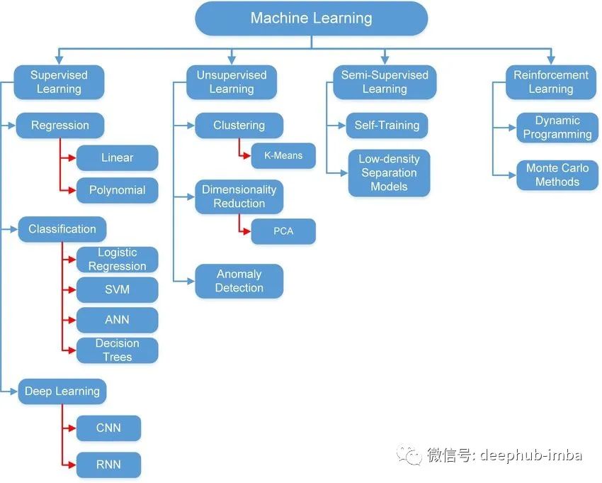
线性回归

Numpy 实现

# Numpy is needed to build the modelimport numpy as np# Import the module matplotlib for visualizing the dataimport matplotlib.pyplot as plt

# We use this line to make the code reproducible (to get the same results when running)np.random.seed(42)# First, we should declare a variable containing the size of the training set we want to generateobservations = 1000
# Let us assume we have the following relationship# y = 13x + 2# y is the output and x is the input or feature# We generate the feature randomly, drawing from an uniform distribution. There are 3 arguments of this method (low, high, size).# The size of x is observations by 1. In this case: 1000 x 1.x = np.random.uniform(low=-10, high=10, size=(observations,1))
# Let us print the shape of the feature vectorprint (x.shape)

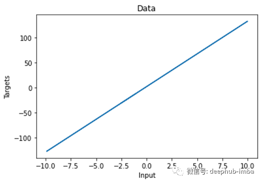
np.random.seed(42)# We add a small noise to our function for more randomnessnoise = np.random.uniform(-1, 1, (observations,1))
# Produce the targets according to the f(x) = 13x + 2 + noise definition.# This is a simple linear relationship with one weight and bias.# In this way, we are basically saying: the weight is 13 and the bias is 2.targets = 13*x + 2 + noise
# Check the shape of the targets just in case. It should be n x m, where n is the number of samples# and m is the number of output variables, so 1000 x 1.print (targets.shape)

# Plot x and targetsplt.plot(x,targets)
# Add labels to x axis and y axisplt.ylabel('Targets')plt.xlabel('Input')
# Add title to the graphplt.title('Data')
# Show the plotplt.show()

np.random.seed(42)# We will initialize the weights and biases randomly within a small initial range.# init_range is the variable that will measure that.init_range = 0.1
# Weights are of size k x m, where k is the number of input variables and m is the number of output variables# In our case, the weights matrix is 1 x 1, since there is only one input (x) and one output (y)weights = np.random.uniform(low=-init_range, high=init_range, size=(1, 1))
# Biases are of size 1 since there is only 1 output. The bias is a scalar.biases = np.random.uniform(low=-init_range, high=init_range, size=1)
# Print the weights to get a sense of how they were initialized.# You can see that they are far from the actual values.print (weights)print (biases)
[[-0.02509198]][0.09014286]

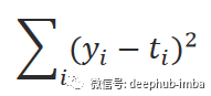
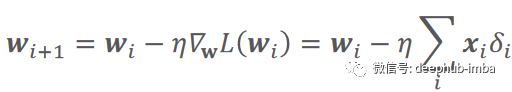
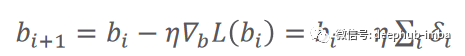
# Set some small learning rate# 0.02 is going to work quite well for our example. Once again, you can play around with it.# It is HIGHLY recommended that you play around with it.learning_rate = 0.02
# We iterate over our training dataset 100 times. That works well with a learning rate of 0.02.# We call these iteration epochs.# Let us define a variable to store the loss of each epoch.losses = []for i in range (100):
   # This is the linear model: y = xw + b equation   outputs = np.dot(x,weights) + biases   # The deltas are the differences between the outputs and the targets   # Note that deltas here is a vector 1000 x 1   deltas = outputs - targets
   # We are considering the L2-norm loss as our loss function (regression problem), but divided by 2.   # Moreover, we further divide it by the number of observations to take the mean of the L2-norm.   loss = np.sum(deltas ** 2) / 2 / observations
   # We print the loss function value at each step so we can observe whether it is decreasing as desired.   print (loss)
   # Add the loss to the list   losses.append(loss)
   # Another small trick is to scale the deltas the same way as the loss function   # In this way our learning rate is independent of the number of samples (observations).   # Again, this doesn't change anything in principle, it simply makes it easier to pick a single learning rate   # that can remain the same if we change the number of training samples (observations).   deltas_scaled = deltas / observations
   # Finally, we must apply the gradient descent update rules.   # The weights are 1 x 1, learning rate is 1 x 1 (scalar), inputs are 1000 x 1, and deltas_scaled are 1000 x 1   # We must transpose the inputs so that we get an allowed operation.   weights = weights - learning_rate * np.dot(x.T,deltas_scaled)   biases = biases - learning_rate * np.sum(deltas_scaled)
   # The weights are updated in a linear algebraic way (a matrix minus another matrix)   # The biases, however, are just a single number here, so we must transform the deltas into a scalar.   # The two lines are both consistent with the gradient descent methodology.

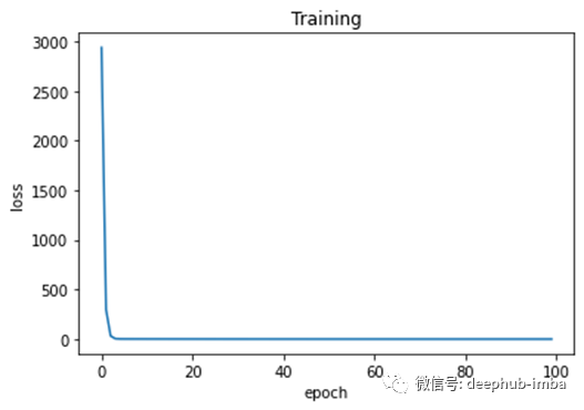
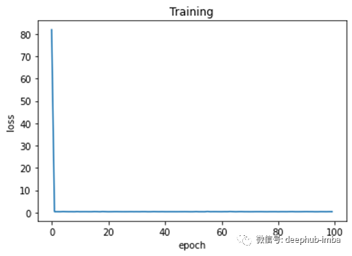
# Plot epochs and lossesplt.plot(range(100),losses)
# Add labels to x axis and y axisplt.ylabel('loss')plt.xlabel('epoch')
# Add title to the graphplt.title('Training')
# Show the plot# The curve is decreasing in each epoch, which is what we need# After several epochs, we can see that the curve is flattened.# This means the algorithm has converged and hence there are no significant updates# or changes in the weights or biases.plt.show()

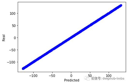
# We print the real and predicted targets in order to see if they have a linear relationship.# There is almost a total match between the real targets and predicted targets.# This is a good signal of the success of our machine learning model.plt.plot(outputs,targets, 'bo')plt.xlabel('Predicted')plt.ylabel('Real')plt.show()
# We print the weights and the biases, so we can see if they have converged to what we wanted.# We know that the real weight is 13 and the bias is 2print (weights, biases)

[[13.09844702]] [1.73587336]

Keras 实现

# Numpy is needed to generate the dataimport numpy as np# Matplotlib is needed for visualizationimport matplotlib.pyplot as plt# TensorFlow is needed for model buildimport tensorflow as tf

np.savez('TF_intro', inputs=x, targets=targets)

# Declare a variable where we will store the input size of our model# It should be equal to the number of variables you haveinput_size = 1# Declare the output size of the model# It should be equal to the number of outputs you've got (for regressions that's usually 1)output_size = 1
# Outline the model# We lay out the model in 'Sequential'# Note that there are no calculations involved - we are just describing our networkmodel = tf.keras.Sequential([                           # Each 'layer' is listed here                           # The method 'Dense' indicates, our mathematical operation to be (xw + b)                           tf.keras.layers.Input(shape=(input_size , )),                           tf.keras.layers.Dense(output_size,                                                # there are extra arguments you can include to customize your model                                                # in our case we are just trying to create a solution that is                                                # as close as possible to our NumPy model                                                # kernel here is just another name for the weight parameter                                                kernel_initializer=tf.random_uniform_initializer(minval=-0.1, maxval=0.1),                                                bias_initializer=tf.random_uniform_initializer(minval=-0.1, maxval=0.1)                                                )                          ])
# Print the structure of the modelmodel.summary()

# Load the training data from the NPZtraining_data = np.load('TF_intro.npz')
# We can also define a custom optimizer, where we can specify the learning ratecustom_optimizer = tf.keras.optimizers.SGD(learning_rate=0.02)
# 'compile' is the place where you select and indicate the optimizers and the loss# Our loss here is the mean square errormodel.compile(optimizer=custom_optimizer, loss='mse')
# finally we fit the model, indicating the inputs and targets# if they are not otherwise specified the number of epochs will be 1 (a single epoch of training),# so the number of epochs is 'kind of' mandatory, too# we can play around with verbose; we prefer verbose=2model.fit(training_data['inputs'], training_data['targets'], epochs=100, verbose=2)

我们可以在训练期间监控每个 epoch 的损失，看看是否一切正常。训练完成后，我们可以打印模型的参数。显然，模型已经收敛了与实际值非常接近的参数值。

# Extracting the weights and biases is achieved quite easilymodel.layers[0].get_weights()
# We can save the weights and biases in separate variables for easier examination# Note that there can be hundreds or thousands of them!weights = model.layers[0].get_weights()[0]
bias = model.layers[0].get_weights()[1]bias,weights
(array([1.9999999], dtype=float32), array([[13.1]], dtype=float32))

PyTorch 实现

# Numpy is needed for data generationimport numpy as np# Pytorch is needed for model buildimport torch

# TensorDataset is needed to prepare the training data in form of tensorsfrom torch.utils.data import TensorDataset
# To run the model on either the CPU or GPU (if available)device = 'cuda' if torch.cuda.is_available() else 'cpu'
# Since torch deals with tensors, we convert the numpy arrays into torch tensorsx_tensor = torch.from_numpy(x).float()y_tensor = torch.from_numpy(targets).float()
# Combine the feature tensor and target tensor into torch datasettrain_data = TensorDataset(x_tensor , y_tensor)

# Initialize the seed to make the code reproducibletorch.manual_seed(42)
# This function is for model's parameters initializationdef init_weights(m):   if isinstance(m, torch.nn.Linear):       torch.nn.init.uniform_(m.weight , a = -0.1 , b = 0.1)       torch.nn.init.uniform_(m.bias , a = -0.1 , b = 0.1)
# Define the model using Sequential class# It contains only a single linear layer with one input and one outputmodel = torch.nn.Sequential(torch.nn.Linear(1 , 1)).to(device)
# Initialize the model's parameters using the defined function from abovemodel.apply(init_weights)
# Print the model's parametersprint(model.state_dict())
# Specify the learning ratelr = 0.02
# The loss function is the mean squared errorloss_fn = torch.nn.MSELoss(reduction = 'mean')
# The optimizer is the stochastic gradient descent with a certain learning rateoptimizer = torch.optim.SGD(model.parameters() , lr = lr)

我们将使用小批量梯度下降训练模型。DataLoader 负责从训练数据集创建批次。训练类似于keras的实现，但使用不同的语法。关于 Torch训练有几点补充：

• 模型和批次必须在同一设备（CPU 或 GPU）上。

• 模型必须设置为训练模式。

• 始终记住在每个 epoch 之后将梯度归零以防止累积（对 epoch 的梯度求和），这会导致错误的值。

# DataLoader is needed for data batchingfrom torch.utils.data import DataLoader
# Training dataset is converted into batches of size 16 samples each.# Shuffling is enabled for randomizing the datatrain_loader = DataLoader(train_data , batch_size = 16 , shuffle = True)
# A function for training the model# It is a function of a function (How fancy)def make_train_step(model , optimizer , loss_fn): def train_step(x , y):   # Set the model to training mode   model.train()   # Feedforward the model with the data (features) to obtain the predictions   yhat = model(x)   # Calculate the loss based on the predicted and actual targets   loss = loss_fn(y , yhat)   # Perform the backpropagation to find the gradients   loss.backward()   # Update the parameters with the calculated gradients   optimizer.step()   # Set the gradients to zero to prevent accumulation   optimizer.zero_grad()   return loss.item() return train_step
# Call the training functiontrain_step = make_train_step(model , optimizer , loss_fn)
# To store the loss of each epochlosses = []
# Set the epochs to 100epochs = 100
# Run the training function in each epoch on the batches of the data# This is why we have two for loops# Outer loop for epochs# Inner loop for iterating through the training data batchesfor epoch in range(epochs): # To accumulate the losses of all batches within a single epoch batch_loss = 0 for x_batch , y_batch in train_loader:   x_batch = x_batch.to(device)   y_batch = y_batch.to(device)   loss = train_step(x_batch , y_batch)   batch_loss = batch_loss + loss # 63 is not a magic number. It is the number of batches in the training set # we have 1000 samples and the batch size is 16 (defined in the DataLoader) # 1000/16 = 63 epoch_loss = batch_loss / 63 losses.append(epoch_loss)
# Print the parameters after the training is doneprint(model.state_dict())
OrderedDict([('0.weight', tensor([[13.0287]], device='cuda:0')), ('0.bias', tensor([2.0096], device='cuda:0'))])

作为最后一步，我们可以绘制 epoch 上的训练损失以观察模型的性能。如图 6 所示。

总结